
](http://esscommunity.org/aiml-blogs/images/global_embeddings.png)
Note: If you haven’t already, I recommend checking out the “Foundation Models for the Earth System: AI that Understands our Planet” post by Phong Le, which introduces the types of models that create these datasets.
What are Geospatial Embeddings?
In the field of satellite remote sensing, advances in artificial intelligence (AI) are reshaping how we search, process, and analyze Earth Observation (EO) data. The 2020s have seen a breakthrough with the rise of Geospatial Foundation Models (GFMs): large neural networks pre-trained on massive catalogs of satellite data and often on many other geospatial data sources.
Using self-supervised learning (SSL) techniques, these models learn general-purpose representations of Earth’s surface. Initially, many applications of these generalist models have involved fine-tuning: customizing the model with your own training data for a specific task, like mapping all water in an image or detecting changes in croplands from year to year. This involves updating the model weights to be more specific to your application.
But beyond their ability to be fine-tuned for specific downstream applications, many of these models also produce embeddings.
Embeddings are an output of foundation model pre-training. At their most basic level, they are vectors: sequences of numbers that represent more complex data. An embedding can compress months or years of multi-source satellite and geospatial data into a compact numerical representation for a single location.
I once heard embeddings jokingly compared to a parent bird feeding its young: the model has already collected and broken down the raw data, then hands us something easier to digest. Crude, but it gets the point across.
In practice, embeddings compress large, complex geospatial datasets, often combining many data types, sensors, and time periods, into a few numbers. That makes them easier to download, analyze, and plug into workflows than if we had to collect, process, and stitch together all the source data ourselves. Moreover, these embeddings exist in a shared latent space, where similar places tend to be closer together numerically.
Latent space is a compressed, abstract representation where high-dimensional data (like images or text) is encoded into a lower-dimensional mathematical space that captures key features and patterns.
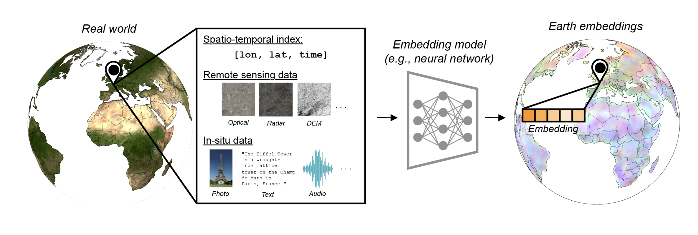
Geospatial embeddings combine diverse inputs, including location, time, satellite data, and in-situ observations like text, photos, and audio, into compact vectors that represent specific places on Earth. Source: Klemmer et al., 2025
Before moving on, it’s important to distinguish between GFMs and embeddings.
- A GFM is something you run. It is the architecture plus the trained weights, and using it typically means setting up an inference pipeline, feeding in input data, and often using GPU resources.
- Embeddings, by contrast, are a static, precomputed data product: a “frozen” output generated by the GFM1. That is one of their biggest advantages. Embeddings separate the heavy computational cost of running a large model from the end user, making the data much easier to digest and plug into downstream workflows.
Many GFM developers are now distributing embeddings from their models as a standalone dataset. Of course, you can also compute embeddings yourself with a GFM, especially if you need a specific time period or custom input data.
Embeddings as a Data Product
So what does an embedding actually look like?
To illustrate this, I’m going to use Google’s AlphaEarth embedding dataset 2, which is publicly available on Google Earth Engine and on Source Cooperative. Below, you can see a visualization of these embeddings for a 10 km area in Alaska’s Arctic coastal plain, a region dotted with wetlands and lakes.
Google’s AlphaEarth embeddings are distributed at an annual time scale and 10-meter pixel resolution. For each 10-meter pixel, in each year, the dataset provides a 64-dimensional vector, in other words, 64 numbers that summarize what the model has learned about that location.
To someone familiar with satellite data, this basically looks like an image with 64 bands when downloaded as a GeoTIFF, except instead of each band representing different wavelengths of the electromagnetic spectrum (red, green, blue, etc.), each band is part of the model’s learned representation of that place.
These embeddings are meant to be used in place of more conventional image composites and engineered features like spectral indices in downstream models. But, similar to the GFMs that produce them, they are generalist datasets. There currently isn’t one embedding dataset specifically meant for hydrology, another for vegetation, and so on. Instead, these datasets are designed to generalize across a wide variety of applications and provide a strong base from which smaller, lighter task-specific models can be trained at a fraction of the time and cost compared to fine-tuning the GFM itself.
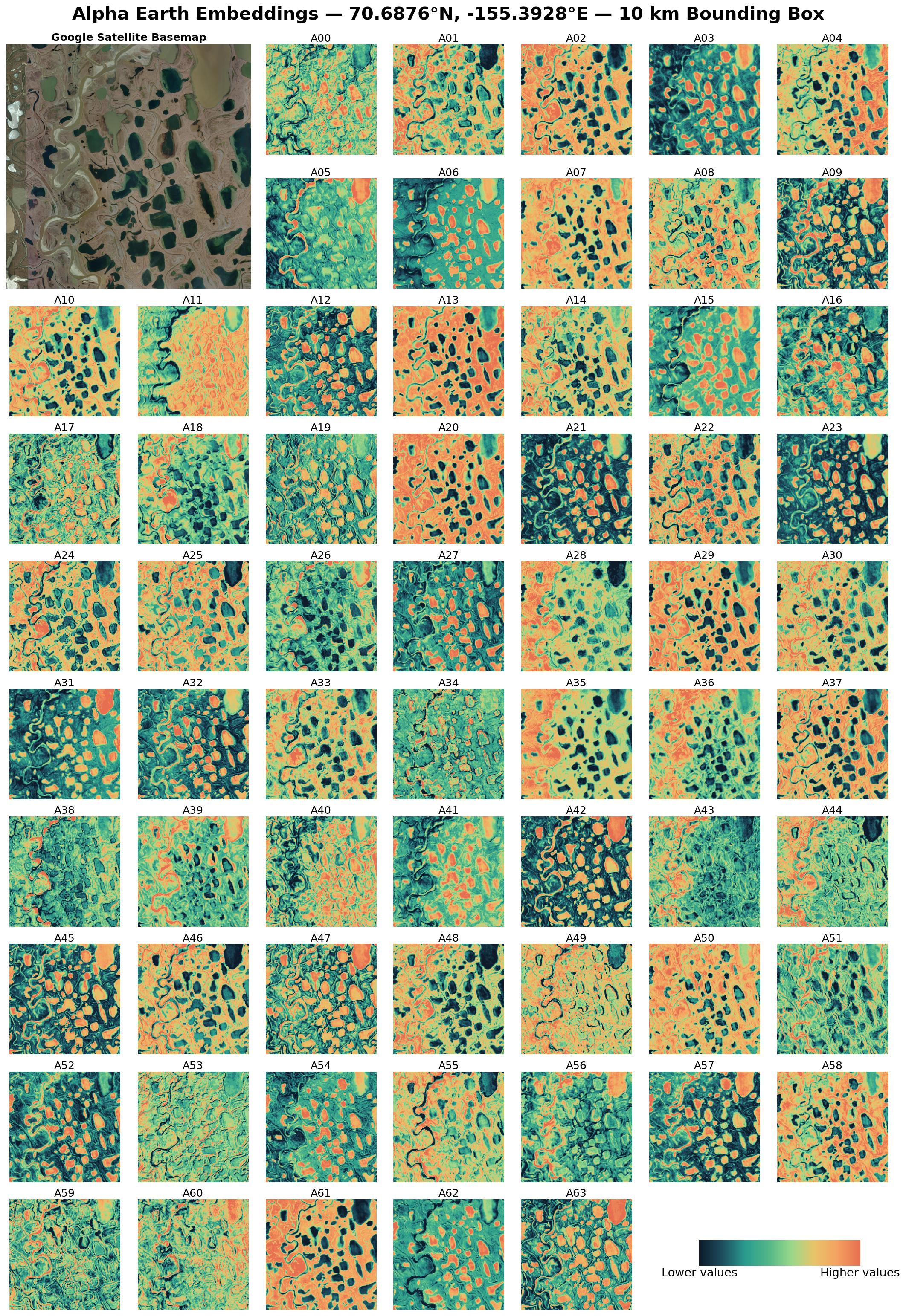
Visualizing Google’s AlphaEarth Embeddings: an example of Google’s AlphaEarth 64-dimensional embeddings for a small area in Alaska’s Arctic coastal plain with clear streams, lakes, and ponds. Data values are in the range of -1 to 1 for each dimension, while each plot shown in this figure is stretched to the min and max of values contained within that subset to clearly visualize the patterns that each dimension highlights.
Many models that produce embeddings are trained using a variety of geospatial datasets, some of which are shown in Table 1 below. A key thing to note is that there is a difference between the data a model learns from during (pre-)training and the data it actually needs at inference time.
Pre-Training: teaches the model what Earth looks like
Inference: asks the model to apply that knowledge to new data
Most end users will not need to compute embeddings themselves, but it is useful to understand the logic behind this distinction. For instance, Google’s AlphaEarth learns from a broad range of inputs, including Sentinel-1/2, Landsat, ERA5 climate data, GEDI vegetation height, L-band radar from PALSAR-2, and others. But once trained, the model does not need all of that information to produce an embedding. At inference time, it only needs Sentinel-1/2, and Landsat 8/9 imagery to generate an annual embedding.
This distinction matters, especially when choosing a specific embedding dataset to work with. Suppose we want to map flooded areas beneath tree canopy, which is notoriously difficult to detect with optical imagery or C-band radar alone. Because AlphaEarth saw L-band radar during training, a data source that can better penetrate canopy cover, it may have learned useful representations associated with inundation under trees. At inference time, even when only optical and C-band inputs are provided, the model may still benefit from those learned relationships, producing embeddings that carry richer context than the inference inputs alone might suggest.
But this has limits. The model cannot recreate L-band-specific signals that were never part of the input. Having the learned context is powerful, but it is not the same as having the raw measurement.
Table 1. Example embedding datasets and their specifications.
| Model | Training Data | Inference Data | Type | Dimensions |
|---|---|---|---|---|
| Google AlphaEarth2 | Sentinel-1/2, Copernicus DEM, ERA5, Landsat, GEDI, GRACE, NLCD, ALOS PALSAR ScanSAR, Wikipedia articles, GBIF | Sentinel-1/2 and Landsat | Pixel | 64 |
| OlmoEarth3 | Sentinel-1/2, Landsat, WorldCover, OpenStreetMap, CDL, WorldCereal, SRTM, Canopy Height | Sentinel-1/2, Landsat | Patch | Varies by model version (128-1024) |
| TESSERA4 | Sentinel-1/2 | Sentinel-1/2 | Pixel | 128 |
| Clay5 | Landsat, Sentinel-1/2, NAIP, LIN, MODIS | Sentinel-2/Sensor Agnostic | Patch | Varies by model version (768-1024) |
Embedding datasets also vary in how many dimensions each vector has — basically, how many numbers are used to represent each location.
AlphaEarth produces a 64-dimensional vector, while OlmoEarth’s largest model produces an embedding dataset with a 1024-dimensional vector, and other models use still different sizes. But bigger does not always mean better. More dimensions do not necessarily mean more useful information; many embedding datasets contain a good amount of redundancy.
For more on this topic, check out this nice blog post by Caleb Robinson and Isaac Corley.
Embedding datasets also differ in whether they are pixel-level or patch-level embeddings. Many early embedding efforts focused on generating a single embedding for each image patch — analogous to an image chip, window, or tile. In other words, one vector might represent a spatial subset read from a larger image, often something like 256 x 256 pixels. Pixel-level embeddings, by contrast, assign an embedding vector to each pixel 1,6.
Pixel Embedding one vector represents each pixel.
Patch Embedding one vector represents a whole image chip/tile/window.
For a nice tutorial on how to do this with AlphaEarth embeddings, check out this link.
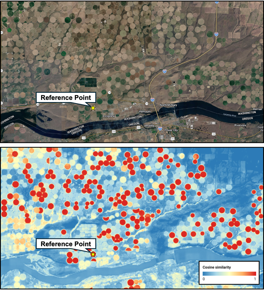
Similarity Search: Example of using a reference point (denoted by the yellow star) to calculate cosine similarity between embedding vectors. Similar vectors appear in red, and vectors that are farther away in embedding space appear in blue.
This is also where embeddings are starting to be adopted in some exciting work combining them with other AI models. Search and retrieval workflows are increasingly being paired with Large Language Models (LLMs), making it possible to query the Earth with plain language. For example, “show me all solar panels in California,” or “find all urban rivers in East Coast cities.” Which is pretty neat compared to manually combing through imagery or maps yourself.
The alternative to patch embeddings is pixel embeddings. These are often the better fit for fine-grained tasks like land cover mapping, flood mapping, or change detection. But “per-pixel” does not mean the model only knows about that one pixel. Depending on the origin model architecture, each pixel’s embedding can still carry information from its neighbors. For example, Google’s AlphaEarth Foundations model produces pixel-based embeddings from a spatiotemporal data cube. It encodes not only a pixel’s behavior through time, but also information about the pixels around it, making the embeddings “spatially aware.”
Overall, if you need high-resolution, more spatially detailed information, pixel-level embeddings are probably going to be your go-to. That said, this is not a firm rule. You can use patch embeddings for segmentation-like tasks, and pixel embeddings for search and retrieval — the similarity example above used embeddings from AlphaEarth, which is pixel-based. The main thing is to understand what each dataset was optimized for and the spatial context that informs each embedding. In fact, many of the patch-based embedding datasets deliver their embeddings at the pixel-level.
Use Cases for Embeddings
We’ve already outlined a few example use cases, but these datasets can support a wide variety of applications. Here is a summary of some of the main ways embeddings are currently being used 6:
Treat embeddings as ready-made features for lightweight models. Instead of starting from raw imagery, you can use embeddings to predict things like agricultural fields, tree cover, species presence, land surface temperature, or other biophysical variables.
Embeddings can give a model a sense of place. They can help condition GeoAI or statistical models to a specific continent, region, ecosystem, or area of interest.
Embeddings can help improve dynamic simulation models by serving as continuous environmental variables, especially where direct observations are sparse. For example, they can provide useful data for hydrologic prediction and forecasting in data-scarce regions.
Embeddings can help make Earth “queryable.” They act like a lookup table for finding similar places or features, like the center-pivot irrigation fields shown earlier.
As these datasets become more explored and adopted into different domain applications, we expect this list of applications to grow as different communities test different datasets.
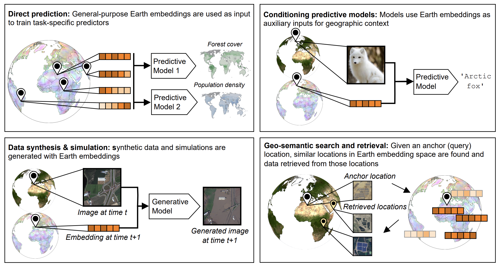
Examples of the diverse applications that geospatial embeddings can be used for. Figure source: Klemmer et al., 2025.
Benefits & Challenges
As with any new data source, there are benefits and challenges to working with geospatial embeddings as they exist today.
Summary
- Geospatial embeddings are compact data products that turn massive, multi-source EO archives into analysis-ready numerical representations.
- Precomputed embeddings lower the barrier to entry, letting users train lighter models for tasks like mapping, change detection, similarity search, and using them as continuous environmental variables in more dynamic modeling applications.
- They are powerful but not a catch-all; there are trade-offs around interpretability, temporal resolution, data size, transparency, and standardization.
- Overall, embeddings offer a pathway to go from dense satellite archives and mixed geospatial datasets to scalable, AI-ready geospatial analytics.
📚 Other Useful Blog Posts if You Want to Learn More
- Geo-Embeddings 101
- How Embeddings Will Revolutionise the Geospatial Data Industry
- Geospatial Embeddings
- Unlocking The Potential of Geospatial Embeddings
- Unlocking the Earth: How AI is Changing the Way We Read Our Planet
- The Hitchhiker's Guide to Vector Embeddings in Machine Learning (for Geographers)
- Geo Embeddings Explained: Understanding Locations as Vectors
- From Earth Pixels to GeoEmbeddings
- How to Actually Use Embeddings
- AI-Powered Pixels: Introducing Google's Satellite Embedding Dataset
🛠️ Resources for Downloading and Using Embeddings
References
Fang, H., et al., 2026. Earth Embeddings as Products: Taxonomy, Ecosystem, and Standardized Access. arXiv preprint arXiv:2601.13134. ↩︎ ↩︎
Brown, C., et al., 2025. AlphaEarth Foundations: An embedding field model for accurate and efficient global mapping from sparse label data. arXiv preprint arXiv:2507.22291. ↩︎ ↩︎
Herzog, H., et al., 2025. OlmoEarth: Stable Latent Image Modeling for Multimodal Earth Observation. arXiv preprint arXiv:2511.13655. ↩︎
Feng, Z., et al., 2025. TESSERA: Temporal Embeddings of Surface Spectra for Earth Representation and Analysis. arXiv preprint arXiv:2506.20380. ↩︎
Klemmer, K., et al., 2025. Earth Embeddings: Towards AI-centric Representations of our Planet. Earth ArXiv preprint https://doi.org/10.31223/X5HX9S. ↩︎ ↩︎