
 (generated with AI via Adobe Stock Images).](http://esscommunity.org/aiml-blogs/images/fox_weather.webp)
- In Part 1, we explored the principles of diffusion models – how they can transform random noise into structured and meaningful data.
- In Part 2, we look at how these models are being applied to weather forecasting and why that shift could make a real difference. If you’re new to diffusion models, we recommend reading Part 1 for useful background context.
Probabilistic Weather Forecasting
Weather affects nearly every aspect of our daily lives – from what we wear in the morning to how we plan for the days ahead. But predicting weather is far from simple because the Earth’s atmosphere is inherently chaotic and highly sensitive to uncertainty.
To address this complexity, scientists rely on ensemble forecasting. Rather than predicting a single deterministic outcome, they run many simulations with slightly different initial conditions. The resulting ensemble provides a range of plausible futures and a quantitative sense of confidence in the forecast.

Tropical cyclone ensemble prediction. Image source: Amanda Montanez
Let’s take tropical cyclones as an example. Predicting the exact path of a storm is notoriously difficult because it depends on many interacting and often unpredictable factors. That’s why forecasters use the cone of uncertainty – the familiar graphic you often see on weather maps. It shows where the storm is most likely headed. As shown in the figure, the forecast is more certain in the near future, and paths at the outside of the cone are less likely than those at the center – but still possible.
Producing these kinds of probabilistic forecasts relies on sophisticated numerical weather prediction (NWP) models. However, these systems demand substantial computing power. Every additional member of the ensemble requires running physics-based simulations, making large ensembles computationally expensive and slow to produce at scale.
Physics-based models use fundamental laws of physics – e.g., conservation of mass, energy, and momentum – to simulate real-world systems. They rely on governing equations, initial/boundary conditions, parameterization, and numerical methods to predict system behavior.
This is where Artificial Intelligence (AI)-based weather forecast models come in. They can produce forecasts much faster – but until recently, they struggled to represent uncertainty in physically meaningful ways. Most AI weather models are trained to produce a single “best guess” forecast, which tends to average away the natural variability of the atmosphere.
That’s beginning to change.
Next-Generation AI for Weather Forecasting
In 2024, Google DeepMind introduced GenCast1, a probabilistic weather forecasting system built on diffusion models. Building on GraphCast2 deterministic architecture, GenCast enhances weather forecasting by quantifying uncertainty and generating many plausible outcomes. It provides:
- Global ensemble forecasts at 0.25$^\circ$ spatial resolution;
- Forecast up to 15 days ahead;
- Improved forecasts for both everyday weather and extreme events compared to ECMWF’s ensemble forecast (ENS).
ECMWF’s ENS is one of the most advanced global weather forecasting systems in the world. It consists of one “best guess” based on the best available input data and 50 additional predictions based on perturbed inputs and model assumptions.
We won’t dive into GenCast’s performance here, as those results are documented in the paper1 and in DeepMind’s blog. Instead, we’ll take a look under the hood and show how GenCast works – breaking down the key ideas in a simple, easy-to-follow way.
Problem Formulation
We begin by explaining how weather forecasting can be framed as a probabilistic modeling problem – and how GenCast uses this framework to generate realistic predictions of future atmospheric conditions.
Let $\mathbf{X}^t$ denote the global weather state at current time $t$. GenCast adopts a second-order Markov approximation for the latent atmospheric dynamics, assuming that the next (unknown) state depends only on the two most recent known states: $$ P(\mathbf{X}^{t+1} \mid \mathbf{X}^{\le t}) \approx P(\mathbf{X}^{t+1} \mid \mathbf{X}^{t}, \mathbf{X}^{t-1}) $$ where $\mathbf{X}^{\le t} = (\dots,\mathbf{X}^{t-1}, \mathbf{X}^{t})$ is the sequence of past weather states up to time $t$.
The task of probabilistic weather forecasting from the present time $t=0$ into the future is to model the joint probability distribution $P(\mathbf{X}^{-1}, \mathbf{X}^{0:T} \mid \mathbf{O}^{\le 0})$, where $T$ is the forecast horizon and $\mathbf{O}^{\le 0}$ are all observations up to the forecast initialization time. This joint probability distribution can be factored as: \begin{aligned} P(\mathbf{X}^{-1}, \mathbf{X}^{0:T} \mid \mathbf{O}^{\le 0}) & = P(\mathbf{X}^{-1}, \underbrace{{\color{red}\mathbf{X}^{0}, \mathbf{X}^{1:T}}}_{\mathbf{X}^{0:T}} \mid {{\mathbf{O}}}^{\le 0}) \\ &\rule{0pt}{1.0em} = P(\mathbf{X}^{0}, \mathbf{X}^{-1} \mid \mathbf{O}^{\le 0}) \times P(\mathbf{X}^{1:T} \mid \mathbf{X}^{0}, \mathbf{X}^{-1}, \mathbf{O}^{\le 0}) \quad \quad \quad \quad {\color{green}\small{\text{Chain rule}}} \\ &\rule{0pt}{1.5em} \approx P(\mathbf{X}^{0}, \mathbf{X}^{-1} \mid \mathbf{O}^{\le 0}) \times {\color{red}P(\mathbf{X}^{1:T} \mid \mathbf{X}^{0}, \mathbf{X}^{-1})} \quad \quad \ \ {\color{green}\small{\text{second-order Markov}}} \\ &\rule{0pt}{1.0em} = \underbrace{P(\mathbf{X}^{0}, \mathbf{X}^{-1} \mid \mathbf{O}^{\le 0})}_{\text{state inference}} \times \underbrace{{\color{red}\prod_{t=0}^{T-1} p(\mathbf{X}^{t+1} \mid \mathbf{X}^t, \mathbf{X}^{t-1})}}_{\text{forecast model}} \quad \ {\color{green}\small{\text{AR(2) factorization}}} \end{aligned}
Model Framework
GenCast models the atmosphere as a high-dimensional dynamical system evolving over space and time. Specifically:
- Each state $\mathbf{X}^t$ consists of 6 surface variables and 6 atmospheric variables at 13 pressure levels on a 0.25$^\circ$ equiangular latitude-longitude grid (i.e., $\mathbf{X}^t \in \mathbb{R}^{(6+6\times 13)\times720\times1440}$).
- Forecasts extend 15 days into the future, with $\Delta t=12$ hour increments between steps, giving $T=30$.
- The state inference represents the probability of the true current state of the atmosphere given available observations up to $t=0$.
- The forecast model calculates the probability of the forecast trajectory $\mathbf{X}^{1:T}$, conditioned on $(\mathbf{X}^{0}, \mathbf{X}^{-1})$, by factoring the joint distribution over successive states – each of which is sampled autoregressively.

Forecast model and trajectory in GenCast. If the current state is at Day 0, 18:00 UTC, the model uses the state from 12 hours earlier (i.e., Day 0, 06:00 UTC) as context to predict the next state at Day 1, 06:00 UTC. Each new predicted state is then fed back into the model to generate subsequent time steps, iteratively progressing through Day 15, 18:00 UTC.
GenCast handles the state inference by simply using existing reanalysis data (ERA5) from ECMWF, including ERA5 EDA (ensemble of data assimilations) for initial conditions. This step is purely numerical and outside the scope of our discussion here.
"Reanalysis data provide the most complete picture currently possible of past weather and climate. They are a blend of observations with past short-range weather forecasts rerun with modern weather forecasting models." – ECMWF
The remaining problem becomes solving the forecast model – and that’s where generative diffusion models step in.
Diffusion Models in GenCast
A key contribution of GenCast is its probabilistic forecast model. At each denoising step, it estimates the conditional probability distribution $p(\mathbf{X}^{t+1} \mid \mathbf{X}^t, \mathbf{X}^{t-1})$ using a diffusion model. This allows GenCast to sample multiple plausible future trajectories, providing a principled representation of forecast uncertainty.
Diffusion models work by first adding random noise to the data, and then learning to remove that noise step by step using a neural network. In Part 1, we described this process using simple Gaussian noise. GenCast, however, extends the idea by sampling noise from a distribution $P_{\text{noise}}(\cdot \mid \sigma)$ that depends on a noise level $\sigma$. Importantly, this noise is applied in the spherical harmonic domain to better respect Earth’s curved geometry and large-scale global weather patterns.
The spherical harmonic domain is a way to represent data on any sphere using smooth, wave-like patterns that cover the whole surface.
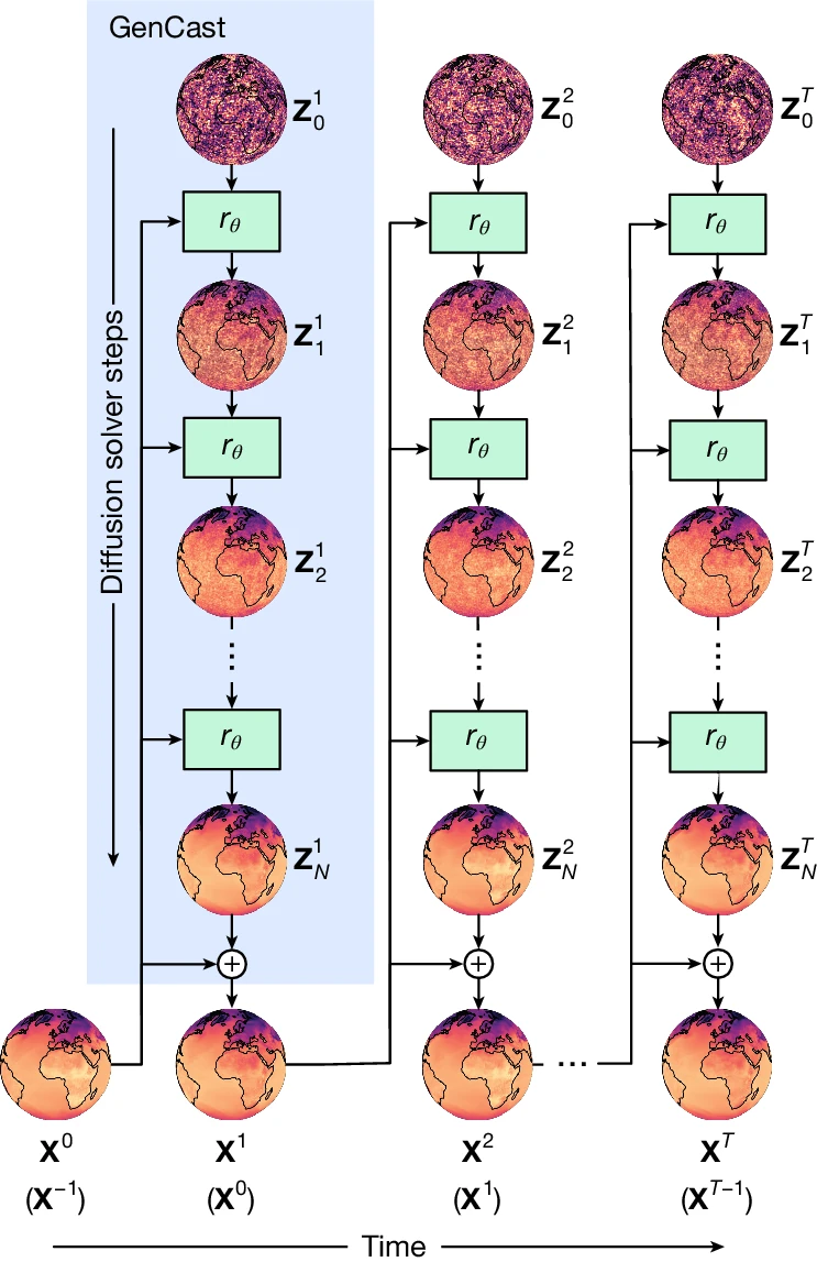
Schematic of how GenCast produces a forecast. The blue box shows how, conditioning on inputs $(\mathbf{X}^{0}, \mathbf{X}^{-1})$, an initial noise sample, $\mathbf{Z}^{1}_0$, is refined by the neural network refinement function, $r_{\theta}$ (green box), which is parameterized by $\theta$. The resulting $\mathbf{Z}^{1}_1$ is the first refined candidate state, and this process repeats N times. The final $\mathbf{Z}^{1}_N$ is then added as a residual to $\mathbf{X}^{0}$ to produce the weather state at the next time step, $\mathbf{X}^{0}.$ This process then repeats autoregressively for $T=30$ times, conditioning on $(\mathbf{X}^{t}, \mathbf{X}^{t-1})$ and using a new initial noise sample $\mathbf{Z}^{t}_0$ at each step to produce the full weather trajectory sample. Each trajectory generated by independent $\mathbf{Z}^{1:T}_0$ noise samples represents a sample from, $P(\mathbf{X}^{1:T} \mid \mathbf{X}^{0}, \mathbf{X}^{-1})$. Image source: Price et al., (2024)
Autoregressive Diffusion Forecast
Once the denoiser in the diffusion model is trained, forecasting becomes a sampling process. At each forecast step, the model turns noise into a physically meaningful weather increment conditioned on the most recent states.
The sampling procedure can be summarized as follows:
- Draw an initial sample $\mathbf{Z}_0^{t+1}$ from a noise distribution $P_{noise}(\cdot \vert \sigma_0)$ on the sphere, at a high initial noise level $\sigma_0$;
- Gradually denoise $\mathbf{Z}_0^{t+1}$ using a refinement function $r_{\theta}$, which applies the denoiser $D_{\theta}$ conditioned on the two most recent states $(\mathbf{X}^0, \mathbf{X}^{-1})$ to obtain $\mathbf{Z}_1^{t+1}$ at lower noise level $\sigma_1<\sigma_0$;
- For $i=1$ to $20$, continue refining $\mathbf{Z}_{i+1}^{t+1} = r_{\theta} (\mathbf{Z}_{i}^{t+1}, \mathbf{X}^{t}, \mathbf{X}^{t-1}, \sigma_{i+1}, \sigma_i)$ until the final residual $\mathbf{Z}^{t+1}=\mathbf{Z}_N^{t+1}$ is obtained at noise level $\sigma_N=0$;
- Update $\mathbf{X}^{t+1} = \mathbf{X}^{t} + S \mathbf{Z}^{t+1}$, where $S$ is a diagonal matrix that inverts the normalization;
- Autoregressively repeat the entire process for 30 times to obtain a full 15-day trajectory forecast.
Notation recap: $t$: forecast time step; $i$: refinement step during noise removal; $\mathbf{Z}_{i}^{t+1}$: weather state increment at step $i$ and time $t+1$; and $\mathbf{X}^t$: full weather state at time $t$
Instead of predicting a single future, GenCast generates many possible futures. Each begins as noise and is gradually shaped into a realistic atmospheric evolution based on learned physics and decades of ERA5 data. For example, 50 different noise samples yield 50 plausible storm paths – some turning north, others speeding up or weakening – capturing the full range of uncertainty in the atmosphere.
ODE solver
In GenCast, the removal of noise is treated as a continuous transformation rather than a series of fixed denoising steps like in DDPMs3. This continuous transformation has a mathematical form called a probability flow ordinary differential equation (ODE). It describes how a noisy sample changes smoothly as the noise level decreases, eventually becoming a clean and physically meaningful weather state.
A useful fact – and the only one we need here – is that this probability flow ODE can be solved just like any other ODEs. GenCast uses a fast numerical method called DPMSolver++2S4 to perform this transformation efficiently. The process is deterministic, requires only a small number of steps, and helps ensure forecasts evolve smoothly and stably over time.
We’ll save the details for another post – the key idea is that this ODE solver enables GenCast to efficiently and accurately transform noise into realistic weather states. Its benefits include:
- Smooth and stable forecast evolution
- Fewer steps needed to refine each sample
- Fast enough to run long forecasts
For more details on the probability flow ODEs, check out this article5.
Denoiser Architecture
The core of the refinement function $r_{\theta}$ is a trainable denoiser neural network $D_{\theta}$. At each step, it reduces noise in the predicted state while enforcing physically realistic atmospheric patterns, ensuring that the evolving forecast remains consistent with large-scale dynamics and fine-scale structures alike.

The architecture of denoiser $D_{\theta}$ in GenCast. The encoder maps local regions of the input into nodes of internal mesh representation. The processor is a graph transformer that updates each node on the mesh. The decoder maps the processed representation from internal mesh back to the grid. The mesh in GenCast is a six-times refined icosahedral mesh. Image source: Lam et al., (2023), Leonhard Döring.
The architecture of $D_{\theta}$ includes 3 main components:
The encoder: maps a noisy target state $\mathbf{Z}_{n}^{t+1}$, as well as the conditioning $(\mathbf{X}^{t}, \mathbf{X}^{t-1})$, from the latitude-longitude grid to an internal learned representation defined on a six-times-refined icosahedral mesh (M$^6$). This mesh helps the model better capture global weather patterns without distortions near the poles.
The processor: is a graph transformer in which each node attends to its k-hop neighborhood on the mesh. It updates each point by learning how weather patterns influence each other across space – helping the model understand spatial features like storms, jet streams, and atmospheric waves.
The decoder: maps the internal mesh representation back to a denoised target state, defined on the grid. The result is a physically meaningful “weather state change” that advances the forecast.
What is icosahedral mesh? An icosahedral mesh is a mesh/grid constructed from an icosahedron – a polyhedron with 20 triangular faces, 12 vertices and 30 edges.

Progressive refinement of icosahedral mesh. GenCast uses a six-times refined icosahedral mesh (M$^6$) with 41,162 nodes and 246,960 edges, which provides a uniform and distortion-limited representation of the global atmosphere. Image adapted from Lam et al., (2023).
Graph transformers are AI models designed for data that naturally form a network – such as weather variables distributed across the globe. They combine the strengths of Transformers6, which excel at capturing long-range dependencies, with Graph Neural Networks (GNNs), which are built to model relationships defined by spatial or structural connectivity.
We’ll explore transformer and GNN architectures – and their applications in Earth sciences – in future posts.
Denoiser Training
During training, we want the denoiser to learn how to remove noise from a future state while still respecting real atmospheric structure. Specifically, the denoiser is applied to a version of the target $\mathbf{Z}^{t+1}$, which has been corrupted by adding noise $\boldsymbol{\varepsilon} \sim P_{noise}(\cdot \vert \sigma)$ at noise level $\sigma$:
$$\mathbf{Y}^{t+1}=D_{\theta }(\mathbf{Z}^{t+1}+\varepsilon;\mathbf{X}^{t},\mathbf{X}^{t-1},\sigma )$$
We train the denoiser to predict $\mathbf{Y}^{t+1}$ as the expectation of the noise-free target $\mathbf{Z}^{t+1}$ through minimization of a loss function: $$ \sum _{t\in {D}_{{\rm{train}}}}\mathbb{E}\left[\lambda (\sigma )\frac{1}{|G| |J| }\sum _{i\in G}\sum _{j\in J}{w}_{j}{a}_{i}{\left({Y}_{i,j}^{t+1}-{Z}_{i,j}^{t+1}\right)}^{2}\right]$$
where:
- $t$: timestep index of the training set $D_{train}$;
- $j \in J$: variable index (include pressure level);
- $i \in G$: location index (latitude and longitude coordinates) in the grid;
- $w_j$: loss weight for variable $j$;
- $a_i$ is the area of the latitude-longitude grid cell;
- $\lambda(\sigma)$ loss weight for noise level $\sigma$.
This loss helps the model learn to remove noise in a physically consistent way across different atmospheric regimes, improving its ability to generalize during forecasting.
The training strategy follows a two-stage resolution approach: the model is first pre-trained at a lower spatial resolution to learn stable, large-scale atmospheric patterns, and then fine-tuned at the full target resolution to capture finer-scale details during the final training phase.
If you’d like to explore the complete Methods in GenCast, check out these papers1,2.
Summary
- Because weather is chaotic, forecasts must quantify uncertainty – and diffusion models offer a powerful, principled way to do exactly that.
- GenCast uses diffusion models to generate fast, high-quality ensemble forecasts up to 15 days ahead.
- GenCast conditions predictions on the last two weather states and iteratively turns noise into future states.
- A specialized architecture (probability flow ODE solver + graph transformer + spherical harmonics) keeps forecasts physically consistent and efficient.
In Part 3, we’ll look at another application of diffusion models for precipitation retrieval from satellite images – stay tuned!
References
Price, I., Sanchez-Gonzalez, A., Alet, F. et al. Probabilistic weather forecasting with machine learning. Nature 637, 84–90 (2025). ↩︎ ↩︎ ↩︎
Lam, R., et al. Learning skillful medium-range global weather forecasting. Science 382, 1416-1421 (2023). ↩︎ ↩︎
Ho, J., Jain, A., & Abbeel, P. (2020). Denoising Diffusion Probabilistic Models. Advances in Neural Information Processing Systems 33 (NeurIPS 2020), pp. 6840-6851. ↩︎
Lu, C. et al., 2022. DPM-Solver++: fast solver for guided sampling of diffusion probabilistic models. ↩︎
Song, J., Meng, C., & Ermon, S., 2020. Denoising diffusion implicit models. arXiv preprint arXiv:2010.02502. ↩︎
Vaswani, A. et al. Attention is all you need. In Advances in Neural Information Processing Systems Vol. 30 (NeurIPS, 2017). ↩︎